Lomb-Scargle Periodograms

The Lomb-Scargle Periodogram (after Lomb [1], and Scargle [2]) is a commonly-used statistical tool designed to detect periodic signals in unevenly-spaced observations. The LombScargle class is a unified interface to several implementations of the Lomb-Scargle periodogram, including a fast O[NlogN] implementation following the algorithm presented by Press & Rybicki [3].

The code here is adapted from the astroml package ([4], [5]) and the gatspy package ([6], [7]).

Basic Usage

Note

All frequencies in LombScargle are not angular frequencies, but rather frequencies of oscillation; i.e. number of cycles per unit time.

The Lomb-Scargle periodogram is designed to detect periodic signals in unevenly-spaced observations. For example, consider the following data:

>>> import numpy as np
>>> rand = np.random.RandomState(42)
>>> t = 100 * rand.rand(100)
>>> y = np.sin(2 * np.pi * t) + 0.1 * rand.randn(100)

These are 100 noisy measurements taken at irregular times, with a frequency of 1 cycle per unit time. The Lomb-Scargle periodogram, evaluated at frequencies chosen automatically based on the input data, can be computed as follows using the LombScargle class:

>>> from astropy.stats import LombScargle
>>> frequency, power = LombScargle(t, y).autopower()

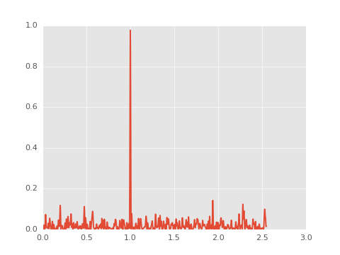
Plotting the result with matplotlib gives:

>>> import matplotlib.pyplot as plt  
>>> plt.plot(frequency, power)       

(Source code, png, hires.png, pdf)

The periodogram shows a clear spike at a frequency of 1 cycle per unit time, as we would expect from the data we constructed.

Measurement Uncertainties

The LombScargle interface can also handle data with measurement uncertainties. For example, if all uncertainties are the same, you can pass a scalar:

>>> dy = 0.1
>>> frequency, power = LombScargle(t, y, dy).autopower()

If uncertainties vary from observation to observation, you can pass them as an array:

>>> dy = 0.1 * (1 + rand.rand(100))
>>> y = np.sin(2 * np.pi * t) + dy * rand.randn(100)
>>> frequency, power = LombScargle(t, y, dy).autopower()

Gaussian uncertainties are assumed, and dy here specifies the standard deviation (not the variance).

Periodograms and Units

The LombScargle interface properly handles Quantity objects with units attached, and will validate the inputs to make sure units are appropriate. For example:

>>> import astropy.units as u
>>> t_days = t * u.day
>>> y_mags = y * u.mag
>>> dy_mags = y * u.mag
>>> frequency, power = LombScargle(t_days, y_mags, dy_mags).autopower()
>>> frequency.unit
Unit("1 / d")
>>> power.unit
Unit(dimensionless)

We see that the output is dimensionless, which is always the case for the standard normalized periodogram (for more on normalizations, see Periodogram Normalizations below).

Specifying the Frequency

With the autopower() method used above, a heuristic is applied to select a suitable frequency grid. By default, the heuristic assumes that the width of peaks is inversely proportional to the observation baseline, and that the maximum frequency is a factor of 5 larger than the so-called “average Nyquist frequency”, computed based on the average observation spacing.

This heuristic is not universally useful, as the frequencies probed by irregularly-sampled data can be much higher than the average Nyquist frequency. For this reason, the heuristic can be tuned through keywords passed to the autopower() method. For example:

>>> frequency, power = LombScargle(t, y, dy).autopower(nyquist_factor=2)
>>> len(frequency), frequency.min(), frequency.max()
(500, 0.0010189890448009111, 1.0179700557561102)

Here the highest frequency is two times the average Nyquist frequency. If we increase the nyquist_factor, we can probe higher frequencies:

>>> frequency, power = LombScargle(t, y, dy).autopower(nyquist_factor=10)
>>> len(frequency), frequency.min(), frequency.max()
(2500, 0.0010189890448009111, 5.0939262349597545)

Alternatively, we can use the power() method to evaluate the periodogram at a user-specified set of frequencies:

>>> frequency = np.linspace(0.5, 1.5, 1000)
>>> power = LombScargle(t, y, dy).power(frequency)

Note that the fastest Lomb-Scargle implementation requires regularly-spaced frequencies; if frequencies are irregularly-spaced, a slower method will be used instead.

Frequency Grid Spacing

One common issue with user-specified frequencies is inadvertently choosing too coarse a grid, such that significant peaks lie between grid points and are missed entirely.

For example, imagine you chose to evaluate your periodogram at 100 points:

>>> frequency = np.linspace(0.1, 1.9, 100)
>>> power = LombScargle(t, y, dy).power(frequency)
>>> plt.plot(frequency, power)   

(Source code, png, hires.png, pdf)

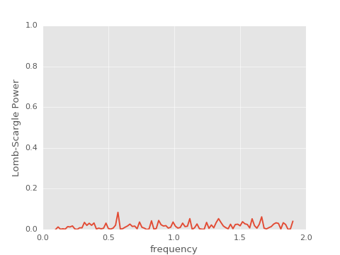
From this plot alone, one might conclude that no clear periodic signal exists in the data. But this conclusion is in error: there is in fact a strong periodic signal, but the periodogram peak falls in the gap between the chosen grid points!

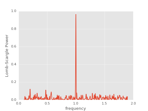
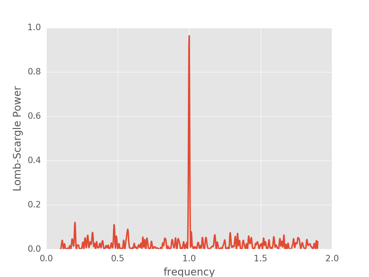
A safer approach is to use the frequency heuristic to decide on the appropriate grid spacing to use, optionally passing a minimum and maximum frequency to the autopower() method:

>>> frequency, power = LombScargle(t, y, dy).autopower(minimum_frequency=0.1,
...                                                    maximum_frequency=1.9)
>>> len(frequency)
884
>>> plt.plot(frequency, power)   

(Source code, png, hires.png, pdf)

With a finer grid (here 884 points between 0.1 and 1.9), it is clear that there is a very strong periodic signal in the data.

By default, the heuristic aims to have roughly five grid points across each significant periodogram peak; this can be increased by changing the samples_per_peak argument:

>>> frequency, power = LombScargle(t, y, dy).autopower(minimum_frequency=0.1,
...                                                    maximum_frequency=1.9,
...                                                    samples_per_peak=10)
>>> len(frequency)
1767

Keep in mind that the width of the peak scales inversely with the baseline of the observations (i.e. the difference between the maximum and minimum time), and the required number of grid points will scale linearly with the size of the baseline.

The Lomb-Scargle Model

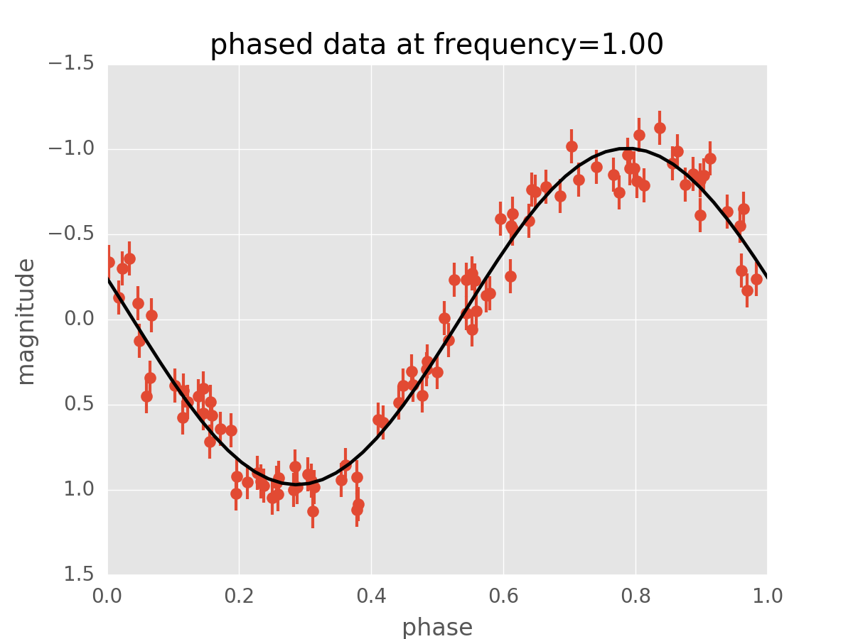
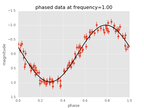
Under the hood, the Lomb-Scargle periodogram essentially fits a sinusoidal model to the data at each frequency, with a larger power reflecting a better fit. With this in mind, it is often helpful to plot the best-fit sinusoid over the phased data.

This best-fit sinusoid can be computed using the model() method of the LombScargle object:

>>> best_frequency = frequency[np.argmax(power)]
>>> t_fit = np.linspace(0, 1)
>>> y_fit = LombScargle(t, y, dy).model(t_fit, best_frequency)

We can then phase the data and plot the Lomb-Scargle model fit:

(Source code, png, hires.png, pdf)

Additional Arguments

On initialization, LombScargle takes a few additional arguments which control the model for the data:

• center_data (True by default) controls whether the y values are pre-centered before the algorithm fits the data. The only time it is really warranted to change the default is if you are computing the periodogram of a sequence of constant values to, e.g. estimate the window power spectrum for a series of observations.
• fit_mean (True by default) controls whether the model fits for the mean of the data, rather than assuming the mean is zero. When fit_mean=True, the periodogram is more robust than the original Lomb-Scargle formalism, particularly in the case of smaller sample sizes and/or data with nontrivial selection bias. In the literature, this model has variously been called the date-compensated discrete Fourier transform, the floating-mean periodogram, the generalized Lomb-Scargle method, and likely other names as well.
• nterms (1 by default) controls how many Fourier terms are used in the model. As seen above, the standard Lomb-Scargle periodogram is equivalent to a single-term sinusoidal fit to the data at each frequency; the obvious generalization is to expand this to a truncated Fourier series with multiple frequencies. While this can be very useful in some cases, in others the additional model complexity can lead to spurious periodogram peaks that outweigh the benefit of the more flexible model.

Periodogram Normalizations

There are several normalizations of the Lomb-Scargle periodogram found in the literature. LombScargle makes four options available, via the normalization argument: normalization='standard' (the default), normalization='model', normalization='log', and normalization='psd'. These normalizations are easiest to discuss in terms of least-squares fits around a constant reference model \(M_{ref}\) and a periodic model \(M(f)\) at each frequency, with best-fit sum-of-residuals that we’ll denote by \(\chi^2_{ref}\) and \(\chi^2(f)\) respectively.

Standard Normalization

The default, the standard normalized periodogram, is normalized by the residuals of the data around the constant reference model:

\[P_{standard}(f) = \frac{\chi^2_{ref} - \chi^2(f)}{\chi^2_{ref}}\]

This form of the normalization (normalization='standard') is the default choice used in LombScargle. The resulting power P is a dimensionless quantity that lies in the range 0 ≤ P ≤ 1.

Model Normalization

Alternatively, the periodogram is sometimes normalized instead by the residuals around the periodic model:

\[P_{model}(f) = \frac{\chi^2_{ref} - \chi^2(f)}{\chi^2(f)}\]

This form of the normalization can be specified with normalization='model'. As above, the resulting power is a dimensionless quantity that lies in the range 0 ≤ P ≤ 1.

Logarithmic Normalization

Another form of normalization is to scale the periodogram logarithmically:

\[P_{log}(f) = \log \frac{\chi^2_{ref}}{\chi^2(f)}\]

This normalization can be specified with normalization='log', and the resulting power is a dimensionless quantity in the range 0 ≤ P ≤ ∞.

PSD Normalization (Unnormalized)

Finally, it is sometimes useful to compute an unnormalized periodogram (normalization='psd'):

\[P_{psd}(f) = \frac{N}{2}\left(\chi^2_{ref} - \chi^2(f)\right)\]

where N is the number of data points, which in the no-uncertainty case will have units y.unit ** 2. This normalization is constructed to be comparable to the standard Fourier power spectral density (PSD):

>>> ls = LombScargle(t_days, y_mags)
>>> frequency, power = ls.autopower(normalization='psd')
>>> power.unit
Unit("mag2")

Note, however, that the normalization='psd' result only has these units if uncertainties are not specified. In the presence of uncertainties, even the unnormalized PSD periodogram will be dimensionless; this is due to the scaling of data by uncertainty within the Lomb-Scargle computation:

>>> # with uncertainties, PSD power is unitless
>>> ls = LombScargle(t_days, y_mags, dy_mags)
>>> frequency, power = ls.autopower(normalization='psd')
>>> power.unit
Unit(dimensionless)

The equivalence of the PSD-normalized periodogram and the Fourier PSD in the unnormalized, no-uncertainty case can be confirmed by comparing results directly for uniformly-sampled inputs. We will first define a convenience function to compute the basic Fourier periodogram for uniformly-sampled quantities:

>>> def fourier_periodogram(t, y):
...     N = len(t)
...     frequency = np.fft.fftfreq(N, t[1] - t[0])
...     y_fft = np.fft.fft(y.value) * y.unit
...     positive = (frequency > 0)
...     return frequency[positive], (1. / N) * abs(y_fft[positive]) ** 2

Next we compute the two versions of the PSD from uniformly-sampled data:

>>> t_days = np.arange(100) * u.day
>>> y_mags = rand.randn(100) * u.mag
>>> frequency, PSD_fourier = fourier_periodogram(t_days, y_mags)
>>> PSD_LS = LombScargle(t_days, y_mags).power(frequency, normalization='psd')

Examining the results, we see that the two outputs match:

>>> from astropy.tests.helper import quantity_allclose
>>> quantity_allclose(PSD_fourier, PSD_LS)
True

This equivalence is one reason the Lomb-Scargle periodogram is considered to be an extension of the Fourier PSD.

For more information on the statistical properties of these normalizations, see e.g. Baluev 2008 [8].

Periodogram Algorithms

The LombScargle class makes available several complementary implementations of the Lomb-Scargle Periodogram, which can be selected using the method keyword of the Lomb-Scargle power. By design all methods will return the same results (some approximate), and each has its advandages and disadganvages.

For example, to compute a periodogram using the fast chi-square method of Palmer (2009) [9], you can specify method='fastchi2':

>>> frequency, power = LombScargle(t, y).autopower(method='fastchi2')

There are currently six methods available in the package:

method='auto'

The auto method is the default, and will attempt to select the best option from the following methods using heuristics driven by the input data.

method='slow'

The slow method is a pure-Python implementation of the original Lomb-Scargle periodogram ([1], [2]), enhanced to account for observational noise, and to allow a floating mean (sometimes called the generalized periodogram; see e.g. [10]). The method is not particularly fast, scaling approximately as \(O[NM]\) for \(N\) data points and \(M\) frequencies.

method='cython'

The cython method is a cython implementation of the same algorithm used for method='slow'. It is slightly faster than the pure-python implementation, but much more memory-efficient as the size of the inputs grow. The computational scaling is approximately \(O[NM]\) for \(N\) data points and \(M\) frequencies.

method='scipy'

The scipy method wraps the C implementation of the original Lomb-Scargle periodogram which is available in scipy.signal.lombscargle(). This is slightly faster than the slow method, but does not allow for errors in data or extensions such as the floating mean. The scaling is approximately \(O[NM]\) for \(N\) data points and \(M\) frequencies.

method='fast'

The fast method is a pure-Python implementation of the fast periodogram of Press & Rybicki [3]. It uses an extirpolation approach to approximate the periodogram frequencies using a fast Fourier transform. As with the slow method, it can handle data errors and floating mean. The scaling is approximately \(O[N\log M]\) for \(N\) data points and \(M\) frequencies.

method='chi2'

The chi2 method is a pure-Python implementation based on matrix algebra (see, e.g. [7]). It utilizes the fact that the Lomb-Scargle periodogram at each frequency is equivalent to the least-squares fit of a sinusoid to the data. The advantage of the chi2 method is that it allows extensions of the periodogram to multiple Fourier terms, specified by the nterms parameter. For the standard problem, it is slightly slower than method='slow' and scales as \(O[n_fNM]\) for \(N\) data points, \(M\) frequencies, and \(n_f\) Fourier terms.

method='fastchi2'

The fast chi-squared method of Palmer (2009) [9] is equivalent to the chi2 method, but the matrices are constructed using an FFT-based approach similar to that of the fast method. The result is a relatively efficient periodogram (though not nearly as efficient as the fast method) which can be extended to multiple terms. The scaling is approximately \(O[n_f(M + N\log M)]\) for \(N\) data points, \(M\) frequencies, and \(n_f\) Fourier terms.

Summary

The following table summarizes the features of the above algorithms:

method	Computational Scaling	Observational Uncertainties	Bias Term (Floating Mean)	Multiple Terms
"slow"	\(O[NM]\)	Yes	Yes	No
"cython"	\(O[NM]\)	Yes	Yes	No
"scipy"	\(O[NM]\)	No	No	No
"fast"	\(O[N\log M]\)	Yes	Yes	No
"chi2"	\(O[n_fNM]\)	Yes	Yes	Yes
"fastchi2"	\(O[n_f(M + N\log M)]\)	Yes	Yes	Yes

In the Computational Scaling column, \(N\) is the number of data points, \(M\) is the number of frequencies, and \(n_f\) is the number of Fourier terms for a multi-term fit.

Example

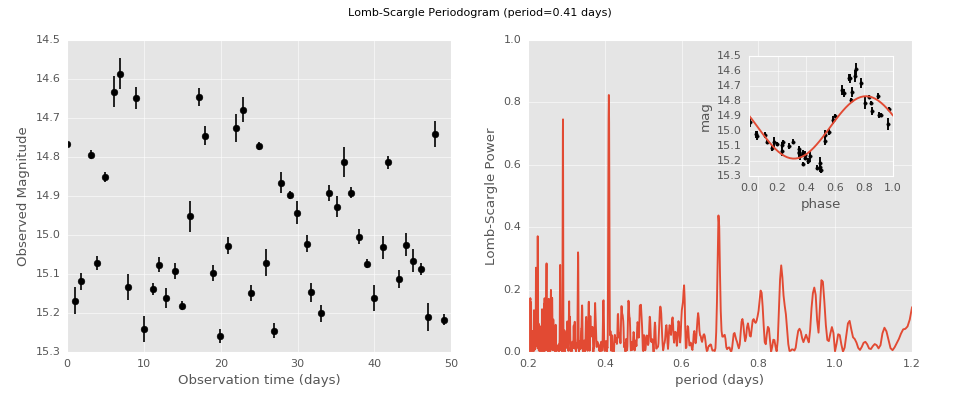
An example of computing the periodogram for a more realistic dataset is shown in the following figure. The data here consist of 50 nightly observations of a simulated RR Lyrae-like variable star, with lightcurve shape that is more complicated than a simple sine wave:

(Source code, png, hires.png, pdf)

This example demonstrates that for irregularly-sampled data, the Lomb-Scargle periodogram can be sensitive to frequencies higher than the average Nyquist frequency: the above data are sampled at an average rate of roughly one observation per night, and the periodogram relatively cleanly reveals the true period of 0.41 days.

Still, the periodogram has many spurious peaks, which are due to several factors:

1. Errors in observations lead to leakage of power from the true peaks.
2. The signal is not a perfect sinusoid, so additional peaks can indicate higher-frequency components in the signal.
3. The observations take place only at night, meaning that the survey window has non-negligible power at a frequency of 1 cycle per day. Thus we expect aliases to appear at \(f_{\rm alias} = f_{\rm true} + n f_{\rm window}\) for integer values of \(n\). With a true period of 0.41 days and a 1-day signal in the observing window, the \(n=+1\) and \(n=-1\) aliases to lie at periods of 0.29 and 0.69 days, respectively: these aliases are prominent in the above plot.

The interaction of these effects means that in practice there is no absolute guarantee that the highest peak corresponds to the best frequency, and results must be interpreted carefully.

Literature References

[1]	(1, 2) Lomb, N.R. Least-squares frequency analysis of unequally spaced data. Ap&SS 39 pp. 447-462 (1976)

[2]	(1, 2) Scargle, J. D. Studies in astronomical time series analysis. II - Statistical aspects of spectral analysis of unevenly spaced data. ApJ 1:263 pp. 835-853 (1982)

[3]	(1, 2) Press W.H. and Rybicki, G.B, Fast algorithm for spectral analysis of unevenly sampled data. ApJ 1:338, p. 277 (1989)

[4]	Vanderplas, J., Connolly, A. Ivezic, Z. & Gray, A. Introduction to astroML: Machine learning for astrophysics. Proceedings of the Conference on Intelligent Data Understanding (2012)

[5]	Vanderplas, J., Connolly, A. Ivezic, Z. & Gray, A. Statistics, Data Mining and Machine Learning in Astronomy. Princeton Press (2014)}

[6]	VanderPlas, J. Gatspy: General Tools for Astronomical Time Series in Python (2015) http://dx.doi.org/10.5281/zenodo.14833

[7]	(1, 2) VanderPlas, J. & Ivezic, Z. Periodograms for Multiband Astronomical Time Series. ApJ 812.1:18 (2015)

[8]	Baluev, R.V. Assessing Statistical Significance of Periodogram Peaks MNRAS 385, 1279 (2008)

[9]	(1, 2) Palmer, D. A Fast Chi-squared Technique for Period Search of Irregularly Sampled Data. ApJ 695.1:496 (2009)

[10]	Zechmeister, M. and Kurster, M. The generalised Lomb-Scargle periodogram. A new formalism for the floating-mean and Keplerian periodograms, A&A 496, 577-584 (2009)